Big Data Mixtape

I grew up within receiving distance of the radio waves of KSHE-95; the country’s oldest FM rock-n-roll radio station. It was my favorite radio station throughout high school and my source for more than a few mix tapes. This was before Spotify, Napster, or even the modern Web as we know it. In fact, not all of my friends even had a computer in their house yet. If you wanted to copy and share music with friends, you had to do it on cassette tapes. I particularly liked to listen to the Monday Night Metal show every Tuesday night on KSHE.

The DJ would play new albums in their entirety without any breaks, which makes for the perfect opportunity to “download” a new album for free. I would have a blank Maxell tape loaded with the record button down and my finger on pause just waiting for the right moment. This is how I obtained my first copy of Metallica’s The Black Album. It may be hard to believe now because Metallica is nearly a household name, but before their seminal Black Album it was rare to hear their music during the day on the airwaves. I don’t remember Lars Ulrich complaining much back then about people recording to cassettes from the radio and sharing with their friends to build their fan base.

Over the years my music collection evolved from Cassette Tapes to CDs. I even acquired a 200 disc CD changer prior to ripping them all to MP3 files. As I think about the progression of various media I’ve used to store my music collection over the years, I’m reminded of the various types of data storage solutions that we have choose from when architecting a data solution. The medium you choose tends to be influenced by how you intend to listen to the data.

Some albums, like Led Zeppelin’s second album, just beg to be listened to from start to finish. I still get frustrated when I don’t hear Livin’ Lovin’ Maid immediately follow Heartbreaker when it’s played on the radio. Sometimes, it is best to listen to your data sequentially too. This is most common when you have a continuous stream of data and you want to do some processing on it. If you “listen” to a stream of clicks on a website, you can count the number of clicks every second and update a dashboard in real-time.

cassette_tape_red_kafka

These streams of data can best be thought of as logs. In fact, the best blog I have read on this is Jay Krep’s article: The Log: What every software engineer should know about real-time data’s unifying abstraction. Jay was one of the principal engineers behind the creation of Apache Kafka whilst at LinkedIn and has since cofounded Confluent to offer a commercial version of software. Apache Kafka is one of the most popular methods to handle the sequential storing and retrieval of data at scale. In fact, the Kafka clusters at Linked in handle hundreds of terabytes of data every day.

A message queue provides a buffer between the system producing the data and the downstream processes that consume it. This buffer becomes important when your consuming system(s) cannot process at the same rate as the data is being produced. If you can scale up your downstream process, then you can increase the rate at which you consume the data. When I used to record music from the radio onto a cassette tape, I was limited by how quickly the music was broadcast over the air. However, whenever I wanted to make a copy for a friend, I could use high-speed dubbing to make a copy on my stereo in about half the amount of time. If you are considering implementing a streaming data solution, you may want to explore some kind of message queue to sequence the data and decouple it from the producers and consumers.

Some albums, and even some artists, don’t beckon to have their entire catalog digested from start to finish. When Pearl Jam came out with Ten, I became an instant fan and bought each new CD they released thereafter. Their B-Sides like Yellow Ledbetter were sometimes better than other bands’ A-Sides. However, by the time I picked up their Yield album, I found myself skipping through tracks.compact_disc_kv

Likewise, if you know exactly which piece of data you want to access quickly, you should consider a key-value store. I knew that if I entered a “key” of 4 after popping in the Pearl Jam’s Yield CD, I would instantly start hearing Given to Fly. When I later entered the album into slot 125 of my CD changer, my “key” became a little bit longer, 125-4. I could still get to the same song even though it was part of a much larger collection. This is the same concept typically used when utilizing a key-value store. The key can have any number of items concatenated together to make it unique.
There are no shortage of key-value stores to choose from. Some of the more popular open source options are Aerospike, Redis, and Riak. A key-value store has no knowledge of what kind of data resides within the “value”, so the responsibility is on the application to know how to interpret the content.

About the same time that my CD collection was outgrowing the limits of my 200 disc changer, I discovered Winamp and MP3 files. One of the great things about MP3 files is that you can record all of the metadata about a song (Artist Name, Album Name, Genre, Year Released, Rating, etc.) in the same file as the audio itself. This allowed me to quickly search the Hair Metal genre and get all of my favorite songs by Cinderella, Def Leppard, Motley Cruë, Poison, Warrant (the list goes on). Essentially, I was doing a reverse lookup on the “values” to retrieve a set of “keys.”Screen Shot 2016-06-04 at 11.15.48 PM

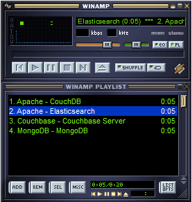
If you need to be able to query your data by some of the entries in the “value”, then you should look at a document data store. These are essentially key-value stores where the “value” has structured data (think JSON or XML) that can be indexed for such queries. The popular open source options in this area are Couchbase, CouchDB, Elasticsearch and MongoDB.

You might be thinking that you don’t need a document data store to create indexes for reverse lookups, because Relational Database Management Systems (RDBMS) like MySQL and Postgres have already been doing this for years. You would be correct too. However, one of the main differences between a document data store and an RDBMS is that the document data store enforces a schema on read, whereas an RDBMS enforces a schema on write. If you decide to start adding another piece of data, such as Mood, you can do so at runtime without invalidating all the documents that came before it. In an RDBMS however, you would need to add a new column to the table’s schema before writing any data to it.  Conversely, one benefit that an RDBMS has, which tends to be lacking in key-value and document data stores, is strict ACID compliance.

So far, all of these examples have been about how I can listen to an individual song, or a set of songs. However, I may want to gleam some insight across my entire music collection. Google has created the Music Timeline to visualize the popularity of various music genres from the 1950s onward.  Search for an individual artist to map their popularity over time.

Screen Shot 2016-06-04 at 11.28.29 PM

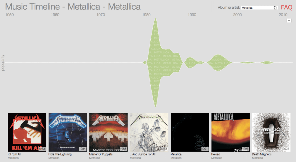
Whenever you need to group large amounts of data with aggregate functions, such as sum() and avg(), you will benefit from using a columnar data store or columnar data format. These data stores are optimized to answer these kinds of summation queries.  The two most popular open source data formats are Parquet and ORC. These files can be easily ingested by query engines such as Spark SQL or Hive.  Alternatively, you may seek to use a columnar data store such as the open source Greenplum.

Through the years, my music library has grown and transitioned from cassette tapes to CDs to MP3s (and even a brief flirtation with MiniDisc).  Likewise, the architecture I have deployed for data solutions has transitioned quite a bit from a standard RDBMS.  There is no wrong way to listen to your music, or your data. Different methods of accessing your collection lend themselves to different mediums, and there’s no shame in duplicating your data across different stores to optimize for different access patterns.  Sometimes you start with one medium and outgrow it for another.  In that spirt, Lars Ulrich will be reassured to know that I did eventually buy The Black Album; on both cassette and CD:)

Deconstructed Data

If you find yourself with a hunger for Greek food in San Francisco, you may want to visit Mezes Kitchen and order a deconstructed gyro.  Rather than presenting the dish as a whole, the individual components of the dish are separated out on the plate to be combined at your whim.

A little over ten years ago the same gastronomical experiment was taking place within Amazon’s engineering department.  The theory was that if you could distill complex applications down to certain “primitives”, then you could more easily compose them into any type of application you want.  These primitives were to be simple, reliable, scalable, and available on-demand.  Elastic Cloud Compute (EC2) and Simple Storage Service (S3) were the first such products to be released in what would come to be known as Amazon Web Services (AWS).  

These primitives serve as the basic building blocks of Compute and Storage that many other products rely on.  One of the main advantages of splitting Compute from Storage is that you can more effectively split the costs from processing and storing your data.  When you pay for S3, you may pay less than $0.03 per Gigabyte per month for storing your data.  The data is automatically replicated several times across multiple data centers and includes durability guarantees of 99.999999999%.  

If some of your data is old and not frequently accessed, but you are not ready to purge it, you can move it to AWS Glacier for a lower cost of $0.007 per Gigabyte per month.  There is no storage requisition process to go through, no limit to the amount of storage you can use, and no people to hire to replace hard drives when they go bad.

As for EC2, there are a number of instance types to choose from which offer various configurations of CPUs, Ram, Storage, and even GPUs.  Some instance types can be rented for a low as a few cents per hour.  Within minutes, you can have a machine available, deployed with the image of your choice for a variety of operating systems.  At any point in time, Amazon has excess capacity in their data centers because all of their servers are not being utilized.  To encourage use, they auction off this excess capacity.  You can bid on instances and pay a “Spot” price which can be much lower than the list price of an on-demand instance.  It’s not uncommon to pay 10% of the on-demand price or less for the same machine.  The only caveat is that your Spot Instance can be taken away from you at any point in time if the Spot price rises above your bid.  To mitigate against this, you can compose clusters with a mixture of on-demand and and spot instances to drive down your overall compute cost.

The result of this on-demand infrastructure allows you to conduct more experiments than you might otherwise had if you were confined to a set number of machines, or if you needed to make a business case for purchasing a large number of machines.  Analytics can now be performed adhoc on data with rented infrastructure to see if it yields value before going through an expensive process to try and fit it into an established data warehouse.

It’s not just infrastructure that has been decomposed into primitives.  Over the past ten years or so, the various components that comprise a traditional database have been split apart to be recomposed at whim.  The engine of a database has retained its familiar SQL interface, but it’s query plan and execution have been replaced by open source projects such as Apache Spark.  The data storage layer has been replaced by object stores, like S3.  This allows the data layer to expand at the same rate that data volume increases, and the compute layer to elastically expand and contract based on the workload being performed.  You can spin up a separate cluster of compute for each department, and shut them down after the employees leave work for the day.  Your ETL jobs can spin up their own clusters and then shutdown immediately after the jobs complete.  Because of this, you can run ETL at the same time as your users’ queries because they aren’t competing for the same resources.

Even the format that data is saved in has gravitated to open source formats that can be read by many different query engines.  This includes column optimized formats like Apache Parquet and ORC.  Large datasets can now be joined together within memory across a cluster of computers.  Each node adds additional CPU and memory to the total capacity.

Compare this to a traditional Data Warehouse built on an RDBMS with 10 years of data.  There needs to be enough storage attached to the server to accommodate all 10 years of data plus extra capacity, which is traditionally planned 6 months to a year in advance.  It’s not uncommon for this storage to be part of an expensive corporate SAN that is shared across various OLAP and OLTP databases.  Anything older than 10 years may need to be archived off to CSV files somewhere with fingers crossed that the online schema doesn’t change too much before it may ever need to be restored.

The RDBMS server itself is probably a single large expensive machine; with an equally sized (and expensive) failover server sitting idle in case the master should fail.  It needs to handle multiple queries from different types of users during the day.  Rarely will those queries access all 10 years of data, but rather only the last year or two.  There may be ETL jobs that run within the database at night, but never during the day because the utilization of the server’s resources may disrupt the queries of business users.  If the data were ever to be migrated from that RDBMS to another data store, you could not simply point a new query engine at them.  You would need to export the data out of the database into some common (but sub-optimal) format like CSV files before importing into the new data store.

In an elastic cloud architecture, there is no limit to the amount of data you can store in S3.  Store 10, 20, 30 years of data!  If you don’t frequently access anything past 10 years, then you could move that older data to AWS Glacier for a cheaper cost.  Storing the data in the Parquet format provides for a compressed columnar representation and schema evolution over time.  Using a query engine, like Spark SQL, allows you to scale out the computation across as many ephemeral clusters as needed; big or small.  Because the data is stored in an open format, you can change query engines if desired without needing to reload data.  There is already a shift underway in migrating older workloads from Apache Hive to Apache Spark.

Amazon is not the only game in town for cloud computing; though they are the biggest and most mature.  Microsoft, Google, IBM, and even Oracle themselves have their own primitives for storage and compute in their respective cloud offerings.  

Whether you have an appetite for gyros or data, you may want to order it deconstructed.  The ability to combine tools at whim from cloud providers and open source software allows you to be more agile with your data solutions.  As you do so, remember to heed the words from another Greek institution, The whole is greater than the sum of its parts.

Apache Spark Scala Library Development with Databricks (or Just Enough SBT)

The movie Toy Story was released in 1995 by Pixar as the first feature-length computer animated film. Even though the animators had professional workstations to work with, they started sketching out the story by hand. A practice that is still followed today for all of Pixar’s films. Whenever you’re developing an Apache Spark application, sometimes you need to sketch it out before you develop it fully and ship it to production.

Follow this link to read the rest of my blog post on Databricks.com

Databricks Lights a Spark Underneath Your SaaS

On January 13, Databricks hosted a meetup in their brand new San Francisco headquarters.  On the agenda was what to expect from their roadmap in 2015.  You can find the entire video here and the slide deck here.

For those who are unfamiliar, Databricks is the company behind the open source software Apache Spark, which is becoming an extremely popular Big Data application engine.  You may have heard of Spark described as being the next generation of Map Reduce, but it is not tied to Hadoop.  Some might say that Spark is in the fast lane to become the killer app for Big Data.  Both the number of patches merged, and the number of contributors has tripled from 2013 to 2014.

At the core of Spark is a concept called Resilient Distributed Datasets (RDD’s).  Without RDD’s, there is no Spark.  An RDD is an immutable, partitioned, collection of elements that can be distributed across a cluster in a manner that is fault tolerant, scales linearly, and is mostly* in-memory. An element can be anything that is serializable.  Working with collections in a language like Java is convenient when the number of elements is in the hundreds or thousands.  However, when that number jumps to millions or billions, you can very quickly run into capacity issues on a single machine.  The beauty of Spark is that this collection can be spread out over an entire cluster of machines (in memory) without the developer needing to think too much about it. Each RDD is immutable and remembers how it was created.  If there is a failure somewhere in the cluster, the failed RDD’s are automatically re-created elsewhere in the cluster.  I prefer to think of it as akin to creating ETL using CREATE TABLE AS statements, except it is not limited to the resources of a single database server.  Nor is it limited to just SQL statements.  If you are curious as to the underpinnings of RDD’s, there is no better resource than to read the 2012 white paper written by its Berkeley creators.

*If the dataset does not fit into memory, Spark can either recompute the partitions that don’t fit into RAM each time they are requested or spill it to disk (added in 2014).

The big takeaway from this meetup is that Databricks is doubling-down on Schema RDD’s to aid with stabilizing their APIs so that they can encourage an strong ecosystem of projects outside of Spark.  A Spark Packages index has already been launched so that developers can create and submit their own packages, much like the ecosystem that already exists for Python and R.  In particular, Spark needs to play catch-up to more established projects by adding machine learning algorithms.  The introduction of Spark Packages will accelerate this.  It was revealed that many Apache Mahout developers have already begun to turn their attention to reengineering their algorithms on Spark.  The Databricks team recognizes that it will be difficult for Spark Packages to reach critical mass without stable APIs.  Therefore, the immediate priority appears to be leveraging Schema RDD’s in both internal and pluggable APIs so that they can graduate them from their Alpha versions.

So what exactly is a Schema RDD?  These were introduced last year as part of Spark SQL, the newest component to the Spark family.  A Schema RDD is “an RDD of Row objects that has an associated schema.”  This is essentially putting structure and types around your data.  Not only does this help to better define interfaces, but it allows Spark to optimize for performance.  Now data scientists can interact with RDDs just like they do with data frames in R and Python.

It wasn’t clear how extensible the meta-data in a Schema RDD will be, or if it will be restricted to basics such as names and types.  This could be a very powerful unifying concept for everything Spark.  In data warehousing, it is not uncommon to build a bespoke solution with Informatica or Data Stage as the ETL engine, Business Objects or Cognos as the BI tool, ER Studio or Embarcadero as the data modeling tool, and a mixture of Oracle, DB2, and SQL Server databases.  Each of these applications has their own catalog of meta-data to manage, and too much of the work involves keeping all of this meta-data in sync.  Schema RDDs have the potential of utilizing a single set of meta-data from the point of sourcing data all the way through to dashboards.

Loading these Schema RDDs from any data source will be accomplished by a new Data Source API.  Data can be sourced into a Schema RDD using a plugin and then manipulated in any supported Spark language (Java, Scala, Python, SQL, R).  The Schema RDD will serve as a common interchange format so that the data can be accessed via Spark SQL, GraphX, MLLib, or Streaming; regardless of which programming language is used.  There are already plugins created for Avro, Cassandra, Parquet, Hive, and JSON.  Support for partitioned data sources will be included in a release later this year so that a predicate can determine which HDFS directories should be accessed.

The Spark Machine Learning Library (MLLib) will leverage Schema RDD’s to ensure interoperability and a stable API.  The main focus for MLLib in 2015 will be the Pipelines API.    This API provides a language for describing the workflows that glue together all the data munging and machine learning necessary in today’s analytics.  There was even a suggestion of partial PMML support for importing and exporting models.  It became apparent that MLLib has some catching up to do when a list of 14+ candidate algorithms for 2015 were projected on the screen along with 5 candidates for optimization primitives.  The sooner all these APIs are stabilized, the sooner the Spark community can get to work on delivering stable packages of these; rather then relying on additions to MLLib itself.  The Pipelines API will become the bridge between prototyping data scientists and production deploying data engineers.

Those were my main takeaways from the prepared remarks.  There were a few interesting discoveries in the Q&A.  A general availability version of Spark R is expected sometime in the first half of this year.  There is a hold up right now due to an incompatible licensing issue.  This project is being driven by Berkeley’s AMP labs rather than Databricks.  There still seems to be more questions than answers about how R is going to fit into the Spark ecosystem other than leveraging Schema RDD’s as data frames.

It was admitted that there is “not much going on” for YARN support in the 2015 roadmap.  Databricks leverages Apache Mesos to administer their clusters, so it is logical to assume their incentive will be to promote Mesos integration as a higher priority.  There are plenty of partners in the Spark ecosystem who are more closely aligned with Hadoop, so I would not be surprised to see one or more of them assuming the mantle for this area.

All of the above is open source and freely available to be installed on your own local cluster.  Databricks is in the business of selling access to their own hosted Spark platform, which has been architected to run on Amazon Web Services.  You can leverage their SaaS solution to have an “instant on” environment for working with Big Data.  Their “Notebooks” interface allows you to write code in a browser and run it interactively.  You can scale clusters up and down on the fly, create data pipelines, and even create dashboards to be published to other users.  From a business intelligence / data analysis point of view, it is very attractive to see how easy it is to analyze data and quickly generate appealing charts.  All of this can be done without the need to install a single server in your data center, or the need to hire a team of people to support the inevitable failure of components.

Ali Ghodsi leads engineering and product management for Databricks, and his theme for his presentation at the 2014 Spark Summit was to pay homage to UI pioneer Alan Kay with their shared desire to “Make simple things simple, and complex things possible.”  This sentence is congruent with the roadmap that was previewed for 2015.  Simple operations such as basic aggregations will become easy to perform with Schema RDDs.  Complex things, such as engineering features as part of a data pipeline to build a gradient boosted decision tree model which is then hosted as part of a real-time data stream, will become possible.  It is still early days, but the excitement around Databricks is catching fire, and as Bruce Springsteen correctly observed, “you can’t start a fire without a spark.”

The Adventures of Mark Twain and Proprietary Hardware

Samuel Clemens, aka Mark Twain, was a celebrated author and humorist, but did you know that he was also a pioneer in Big Data?  As a teenager, young Samuel worked an apprenticeship with a printer as a typesetter.  After earning success with The Adventures of Tom Sawyer he started to invest in a new way of setting type for a printing press.  It was called the Paige Compositor, and it promised to revolutionize the way information would be printed by setting and printing type one line at a time; rather than a character at a time.  This would dramatically increase data velocity for the times.  Mark Twain became an investor in 1877, but the invention never took off.  After 17 years, only 2 production machines had been built, and Mark Twain was forced to file for bankruptcy.  He had failed to follow one of the cardinal rules of wealth management; diversification.

Just as it is not prudent to keep all of your financial eggs in one basket, it is not recommended to keep all of your data resources in a single server.  Big Data doesn’t mean Big Server, but rather it is necessitating that every layer of an application be distributed across multiple nodes.  This includes file systems, message queues, processing, and data stores.  Distributing your computing resources will diversify the risk of system failure and allow easier scalability by adding more nodes; rather than by purchasing increasingly bigger singleton servers.

How many of you have been involved in a data warehouse project where there is an ETL server extracting from a bunch of relational databases, transforming the data, loading it into an even bigger relational database (ODS/DW), which is then queried by some business intelligence tool?  The BI layer can scale by adding more servers.  The more robust ETL tools can scale by adding more servers and partitioning the data.

The one component that can’t be easily distributed across multiple servers is the RDBMS.  Just like a financial portfolio, it is risky to keep most of your assets in one place.  A distributed computer system is only as diversified as its weakest link.  When the database needs to scale, this usually means buying a more powerful (and more expensive) machine.  In my past experiences, more times than not, the database was where my performance bottleneck would be too.  A typical complaint from the business would start with “Informatica is slow.”  However, after delving into the details, the ETL server was either waiting on the source database to read from, or waiting on the target database to write to.  I have been fortunate in my career to work with some extremely talented DBAs who could really make Oracle purr.  At some point though, the data starts to get too big to manage easily within a standard RDBMS.

About 10 years ago, massive parallel processing (MPP) databases and data warehouse appliances were starting to gain attention because of their fast performance and lower cost compared to Teradata.  Data was automatically replicated and disks or nodes could easily be swapped out if there was a hardware failure.  If your data pushed the capacity of the appliance, it could be extended, or a bigger model purchased.  I partnered with Netezza 7 years ago and was very impressed by the performance of their technology at the time.  I bumped into a Netezza user at a conference recently who shared my appreciation for the product, but then added that license costs had doubled after the company was acquired by IBM.  Being acquired was not unique to Netezza.  Here’s a brief timeline of MPP M&A:

2008

  • DATAllegro is acquired by Microsoft in 2008 and rebranded SQL Server Parallel Data Warehouse.

2009

  • Oracle releases its first version of Exadata in conjunction with HP.

2010

  • Netezza is acquired by IBM
  • Greenplum is acquired by EMC and is now part of their Pivotal big data initiative.
  • SybaseIQ is acquired by SAP

2011

  • Aster Data Systems is acquired by Teradata
  • HP retires its homegrown Neoview line in 2011
  • Oracle announces that Exadata will use Sun-based hardware (acquired in 2010)
  • Vertica is acquired by HP

2013

  • ParAccel is acquired by Actian

Some of these use proprietary hardware, while others can be run over a cluster of commodity servers.  In 2012, Amazon chose ParAccel to be the underpinnings behind its RedShift MPP service which manages all the administration behind the scenes and provides the service at $1,000 per terabyte.  There seems to be a bit of an overlap between Hadoop and MPP databases and a common pattern is emerging with Hadoop handling the batch ETL and the MPP database acting as a cache for user queries.  Every vendor is scrambling to tell their own story as to how their MPP database lives in harmony with Hadoop.  I haven’t heard of a new entrant into the MPP appliance space in years.  However, Hadoop appliances are now on the scene from many of the same vendors that acquired the MPP upstarts, and even a few high performance computing manufacturers such as Cray and SGI.  This recent article from InformationWeek does a good job of describing the landscape.

The trend of both Big Data and Cloud Computing is to spend money on lots of cheaper commodity machines, rather than on proprietary hardware.  These cheaper commodity machines, don’t need to be requisitioned and purchased with upfront costs if they are part of a public cloud.  If you want to do a proof of concept, just purchase compute and storage on demand.  HDFS is more than capable of scaling to petabytes of data, and there is increased focus in running SQL like queries against it.  The Apache Spark project seeks to leverage the resources of a commodity cluster to distribute resilient datasets in memory.  Before mapping out a space in your data center for that shiny new piece of expensive hardware, you might want to see how far you can get on commodity boxes.  There will always be a space for specialty hardware for special situations, but is your Big Data use case really that special compared to the common use cases?

Mark Twain was not ill-informed about the trends in publishing.  He had been in and around the industry since he was a teenager, and the Paige Compositor was headed in the right direction of setting type one line at a time.  He just happened to bet on the wrong hardware.  The Linotype machine began taking orders 3 years prior to the Paige Compositor and had locked up the market with its simpler design and exceeding durability.  After 17 years of investment, it cannot be said that Mark Twain was not a patient man.  I think we can all agree that he would have made a better blogger than venture capitalist.  He is quoted with having learned two lessons from the experience: “not to invest when you can’t afford to, and not to invest when you can.”

Three V’s are Enough!

Any man who has been fortunate enough to find that special someone whom he wants to share the rest of his life with, has been through the experience of picking out an engagement ring and therefore become familiar with the 4 C’s.  I’m talking about the Cut, Color, Clarity, and Carat of a diamond.  This was a standard created by the Gemological Institute of America (GIA) in the mid 20th century to standardize on how to describe the quality of diamonds.  It’s a useful way to describe the different aspects of what impacts the value of a diamond in an easy to remember short list of items.  You can tweak each dimension up or down its scale and immediately see the impact to your bank account.

Just as diamonds have a snappy way to describe them, so too does Big Data.  Instead of the 4 C’s, we have the 3 V’s: Volume, Velocity, and Variety.  You can trace the standardization of this definition back to a paper by Doug Laney for the META Group in 2001 titled “3D Data Management: Controlling Data Volume, Velocity, and Variety.”  This paper was written at a time when the seeds for Web 2.0 were being sown, and Doug was mainly referring to the challenges of managing data at web scale.  In addition to DBMS data, this included web logs to track clickstream data.

The definition of the 3 V’s might seem a bit obvious, but I will briefly explain them in this blog post.  The Volume dimension of data is most readily associated with Big Data, just as temperature change is the most known aspect of Global Warming.  Although this is the V that might get the most attention because of it’s “Bigness”, it is probably the least interesting of the dimensions.  The volumes of data to manage has been increasing at an exponential rate, but so too has our ability to process and store it; at a reduced cost.  The cost of disk storage at the time that Doug wrote his paper was roughly $10 per gigabyte.  Today, it is closer to .10 cents per Gigabyte.  I have more (flash) storage on my phone today than the total disk storage I had on my computer back in 2001.

Whoever coined the term Big Data, could have just as easily chosen the term Fast Data to describe this new paradigm.  Had that been the case, then the Velocity dimension would have garnered the same attention that Volume does.  Because data is now being generated at such a fast rate and at such a great volume, it is not acceptable nor feasible to fit this processing into some batch window at the end of the working day.  As a data warehouse architect, I would always encounter the requirement for real-time reporting from the business.  There are various strategies to enable this, but all of them required adding a level of complexity and cost on top of the batch focused ETL infrastructure.  This included staffing up the support team to ensure real-time support when failures occurred.  Sometimes the business got there, but in many cases they determined that the higher costs weren’t justified.  If you architect a system for real-time data processing in the beginning, you can augment it with batch processing for large workloads.  Conversely, if you start with a batch processing system, it is much more difficult to augment or transform it into a real-time data processing system.

Variety is the spice of life and data is no exception.  The world of Big Data does not constrain itself to only structured data residing in relational databases.  Rather, there is no limit to the type of data that can be ingested and analyzed.  This includes documents, photos, audio, and video recordings.  Part of the allure of HDFS is that any type of data can be stored, accessed, and analyzed.  It frees data from the constraints and structure of a database, and pushes down the responsibility of dealing with schemas from the point of writing the data to the point of reading it.

If you’re thinking of experimenting with Big Data and are curious as to what type of initiative may best lend itself to it, think about which of the 3 V’s are the biggest challenges to fitting your initiative into the traditional data warehouse model over a DBMS.  When you need a killer app that can’t be done easily or cheaply with the old way, you may have a good candidate for Big Data.

Most people would agree that these 3 V’s are a reasonable and succinct way to characterize this new paradigm of data.  However, if you follow any Big Data web forums, you’ll find all manner of suggestions for how the 3 V’s should be expanded to include other V’s such as Variability, Verification, Viability, Vision, Validity, and even Virility. I was at a conference where an architect put up a slide with 18 different V words!!  Leave it to architects and engineers to take an easy to comprehend concept and pedantically pick it apart until it completely loses its intended purpose.  My personal favorite is when engineers try to inject some algorithms into the marketing.  I found this gem on a web forum:

    (Volume + Variety + Velocity + Veracity) * Visualization = Value

Einstein is generally regarded as a pretty smart guy, and he managed to distill his theory of relativity down to E = mc2.  Why should data be more complicated than the theory supporting our entire universe?  Let’s all just agree that Doug’s original 3 dimensions of Volume, Velocity, and Variety is sufficient enough to characterize what sets Big Data apart from our traditional notions of data.  If we can make one of the most important purchasing decisions of our lives based upon 4 C’s, then surely we can get by with just 3 V’s to communicate the dimensions of what makes data the most challenging to work with.  When the next major shift in technology presents itself, then we can always come up with a new snappy way to communicate.  After all, diamonds may be forever, but technical paradigms are not.